In this blog series, I’ll walk through my journey optimizing a canonical Conv2D kernel — starting from a deeply nested CPU loop, all the way to handcrafted CUDA kernels that rival cuDNN and CUTLASS.

Motivation
Background: What Does Conv2D Actually Do?
Roofline: Theoretical Peak Performacne
CPU Implementation and Tuning
What’s Next

Motivation

The convolution layer is the cornerstone of modern neural networks. This series documents the engineering path from naive to state-of-the-art implementations of a Conv2D operation — measuring the work, insight, and tooling required to bridge the performance gap.

We chose a canonical configuration:

Input: NHWC shape (10, 224, 224, 128)
Filter: KRSC shape (128, 3, 3, 128)
Output: NPQK shape (10, 224, 224, 128)
Padding: 1, Stride: 1, Dilation: 1

This setup represents a mid-depth convolutional layer common in real-world CNNs (e.g., EfficientNet, ResNet), and its optimization is relevant for both training and inference pipelines.

Background: What Does Conv2D Actually Do?

At its core, a 2D convolution computes weighted dot products over local spatial windows across input channels. Here’s a visualization with a 3×3 kernel. Imagine each 3×3 input patch has a depth of C = 128. Each filter produces a single output value, and we use K = 128 such filters. This gives a filter shape of KRSC = (128, 3, 3, 128).

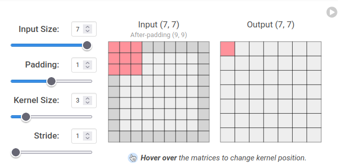
Conv2d visualization. Credit: https://poloclub.github.io/cnn-explainer/

Credit: https://poloclub.github.io/cnn-explainer/

Mathematically, for each output element O[n, p, q, k], we compute:

\[O[n, p, q, k] = \sum_{r = -1}^{1} \sum_{s = -1}^{1} \sum_{c = 0}^{C - 1} I[n, p + r, q + s, c] \cdot W[k, r + 1, s + 1, c]\]

Note: r and s range from -1 to 1 due to centered 3×3 kernels.

Roofline: Theoretical Peak Performance

Before diving into code, we estimate the ideal performance bounds on our hardware to benchmark how close our implementation gets to peak throughput.

We start by analyzing arithmetic intensity (AI) — the ratio of computation to memory traffic. This tells us whether the kernel is compute-bound or memory-bound.

Arithmetic Intensity (AI) Analysis of Conv2D

Total Floating Point Operations (FLOPs)

Each output element performs:

CRS = 128 × 3 × 3 = 1152 multiply-accumulates
Each MAC = 2 FLOPs

Total FLOPs:

\[\text{FLOPs} = N \times P \times Q \times K \times C \times R \times S \times 2 = 147.975 \text{ GFLOPs}\]

Total Memory Accessed

Unique elements accessed:

Input (NHWC): 10 × 224 × 224 × 128 = 64,100,352
Filter (KRSC): 128 × 3 × 3 × 128 = 147,456
Output (NPQK): 10 × 224 × 224 × 128 = 64,100,352

Total: 128,598,160 elements

FP32: 128,598,160 × 4 bytes = 514.39 MB
FP16: 128,598,160 × 2 bytes = 257.20 MB

Arithmetic Intensity (AI)

FP32: 147.975 GFLOPs / 514.39 MB = 287.67 FLOP/byte
FP16: 147.975 GFLOPs / 257.20 MB = 575.34 FLOP/byte

Roofline: CPU vs GPU

CPU: AMD Ryzen 2700

Spec	Value
Cores	8 (SMT disabled)
Clock speed	3.2 GHz
SIMD width	AVX2 (8 FP32 per register)
Peak FLOPs	409.6 GFLOP/s
Mem bandwidth (DDR4-3200)	~51.2 GB/s
Ridge Point	8.0 FLOP/byte

GPU: RTX 2070 Super (CUDA Cores)

Spec	Value
SMs	40
CUDA cores per SM	64
Clock speed	1.8 GHz
Peak FLOPs	9.216 TFLOP/s
Mem bandwidth	448 GB/s
Ridge Point	20.57 FLOP/byte

GPU: RTX 2070 Super (Tensor Cores)

Spec	Value
Tensor cores (40 SMs × 8)	320
Peak FLOPs (FP16)	73.728 TFLOP/s
Ridge Point	164.57 FLOP/byte

Conclusion

In all cases, the kernel AI is well above each device’s ridge point, which means:

The kernel is compute-bound on both CPU and GPU.
We can estimate ideal runtimes by dividing FLOPs by peak device throughput:

Device	Peak FLOP/s	Ideal Time
Ryzen 2700	409.6 GFLOP/s	361 ms
RTX 2070 (CUDA)	9.216 TFLOP/s	16.05 ms
RTX 2070 (Tensor)	73.728 TFLOP/s	2.01 ms

CPU Implementation and Tuning

Naive CPU Kernel (NCHW Layout)

Our initial implementation used NCHW and ran in 150 seconds — far from the ideal 361 ms.

extern "C" void conv2d(float* input, float* weight, 
                       int n,
                       int h, int w, int c_in,
                       int r, int c_out,
                       int stride,
                       int padding,
                       float* z)
{
    int p = (h + 2*padding - r) / stride + 1;
    int q = (w + 2*padding - r) / stride + 1;

    const int r_offset = (r - 1) / 2;
    const int s_offset = (r - 1) / 2;

    for (int n_i = 0; n_i < n; ++n_i) {
        for (int k_i = 0; k_i < c_out; ++k_i) {
            for (int p_i = 0; p_i < p; ++p_i) {
                for (int q_i = 0; q_i < q; ++q_i) {
                    float acc = 0;

                    for (int c_i = 0; c_i < c_in; ++c_i) {
                        for (int r_i = 0; r_i < r; ++r_i) {

                            int h_i = p_i + r_i - r_offset;
                            if (h_i < 0 || h_i >= h) continue;

                            for (int s_i = 0; s_i < r; ++s_i) {

                                int w_i = q_i + s_i - s_offset;
                                if (w_i < 0 || w_i >= w) continue;

                                int input_index = ((n_i * c_in + c_i) * h + h_i) * w + w_i;
                                int weight_index = ((k_i * c_in + c_i) * r + r_i) * r + s_i;

                                acc += input[input_index] * weight[weight_index];
                            }
                        }
                    }

                    int output_index = ((n_i * c_out + k_i) * p + p_i) * q + q_i;
                    z[output_index] = acc;
                }
            }
        }
    }
}

Improving Cache Locality with NHWC

Switching to NHWC and restructuring loops around the innermost C dimension brought runtime down to 23 seconds — a 6.5× speedup due to better memory locality.

extern "C" void conv2d_nhwc(float* __restrict__ input, float* __restrict__ weight, 
                            int n,
                            int h, int w, int c_in,
                            int r, int c_out,
                            int stride,
                            int padding,
                            float* __restrict__ z)
{
    int p = (h + 2*padding - r) / stride + 1;
    int q = (w + 2*padding - r) / stride + 1;

    const int r_offset = (r - 1) / 2;
    const int s_offset = (r - 1) / 2;

    for (int n_i = 0; n_i < n; ++n_i) {
        for (int p_i = 0; p_i < p; ++p_i) {
            for (int q_i = 0; q_i < q; ++q_i) {
                for (int k_i = 0; k_i < c_out; ++k_i) {

                    float acc = 0;

                    for (int r_i = 0; r_i < r; ++r_i) {

                        int h_i = p_i + r_i - r_offset;
                        if (h_i < 0 || h_i >= h) continue;

                        for (int s_i = 0; s_i < r; ++s_i) {

                            int w_i = q_i + s_i - s_offset;
                            if (w_i < 0 || w_i >= w) continue;

                            for (int c_i = 0; c_i < c_in; c_i += 8) {

                                int input_index = ((n_i * h + h_i) * w + w_i) * c_in + c_i;
                                int weight_index = ((k_i * r + r_i) * r + s_i) * c_in + c_i;

                                float tmp_acc = 0;

                                for (int c_offset = 0; c_offset < 8; ++c_offset) {
                                    tmp_acc += input[input_index + c_offset] * weight[weight_index + c_offset];
                                }
                                acc += tmp_acc;
                            }
                        }
                    }

                    int output_index = ((n_i * c_out + k_i) * p + p_i) * q + q_i;
                    z[output_index] = acc;
                }
            }
        }
    }
}

Adding OpenMP Parallelism

By parallelizing over the outer loops (e.g., n, p, q), we utilized 8 physical CPU cores:

    #pragma omp parallel for collapse(2) schedule(static)
    for (int n_i = 0; n_i < n; ++n_i) {
        for (int p_i = 0; p_i < p; ++p_i) {
            for (int q_i = 0; q_i < q; ++q_i) {
                for (int k_i = 0; k_i < c_out; ++k_i) {
                    ...

This further reduced runtime to 3.4 seconds, a 44× overall improvement.

Summary: CPU Conv2D Performance

Version	Layout	Parallelism	Time	Speedup
Naive CPU	NCHW	None	150 s	1×
Naive CPU	NHWC	None	23 s	6.5×
CPU + OMP	NHWC	8 cores	3.4 s	44×

This final CPU implementation achieved about 11% of theoretical peak, which is quite reasonable for a memory-coordinated workload without heavy vectorization or compiler intrinsics.

What’s next?

In Part 2, we’ll explore cuDNN and CUTLASS baselines on the GPU, and eventually challenge them with our own hand-rolled CUDA kernels.

The big question: How hard is it to get from 3.4 seconds down to 2.01 ms

Optimizing Conv2D from Scratch: CPU to GPU Journey (Part 1)

Table of Contents